Social Network Analysis Using R

R is a programming language and an environment for statistical computing. R development takes advantage of a growing community that cooperates in its development due to its open source philosophy.

In effect, the source code of every R component is freely available for inspection and/or adaptation.This fact allows you to check and test the reliability of anything you use in R. R does though have limitations with handling enormous datasets because all computation is carried out in the main memory of the computer.

This does not mean that we will not be able to handle these problems. Taking advantage of the highly flexible database interfaces available in R like MySQL, we will be able to perform data mining on large problems.

Case Study of social network analysis with R:

Load Data

> # load termDocMatrix > load(“data/termDocMatrix.rdata”) > # inspect part of the matrix > termDocMatrix[5:10,1:20]

Note that the above term DocMatrix is a standard matrix, instead of a term-document matrix under the framework of text mining. To try the code with your own term-document matrix built with the tm package, you need to run the code below before going to the next step.

> termDocMatrix <- as.matrix(termDocMatrix)

Transform Data into an Adjacency Matrix

> # change it to a Boolean matrix > termDocMatrix[termDocMatrix>=1] <- 1 > # transform into a term-term adjacency matrix > termMatrix <- termDocMatrix %*% t(termDocMatrix) > # inspect terms numbered 5 to 10 > termMatrix[5:10,5:10]

Build a Graph

Now we have built a term-term adjacency matrix, where the rows and columns represents terms, and every entry is the number of co-occurrences of two terms. Next we can build a graph with graph.adjacency() from package igraph.

> library(igraph) > # build a graph from the above matrix > g <- graph.adjacency(termMatrix, weighted=T, mode = “undirected”) > # remove loops > g <- simplify(g) > # set labels and degrees of vertices > V(g)$label <- V(g)$name > V(g)$degree <- degree(g)

Plot the Graph

> # set seed to make the layout reproducible > set.seed(3952) > layout1 <- layout.fruchterman.reingold(g) > plot(g, layout=layout1)

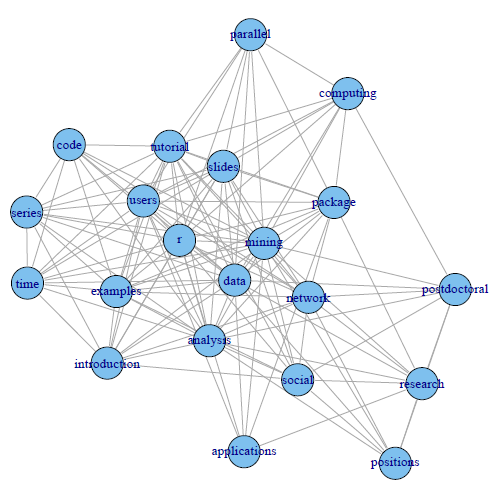
A different layout can be generated with the first line of code below. The second line produces an interactive plot, which allows us to manually rearrange the layout. Details about other layout options can be obtained by running? igraph::layout in R.

> plot(g, layout=layout.kamada.kawai) > tkplot(g, layout=layout.kamada.kawai)

Make it Look Better!

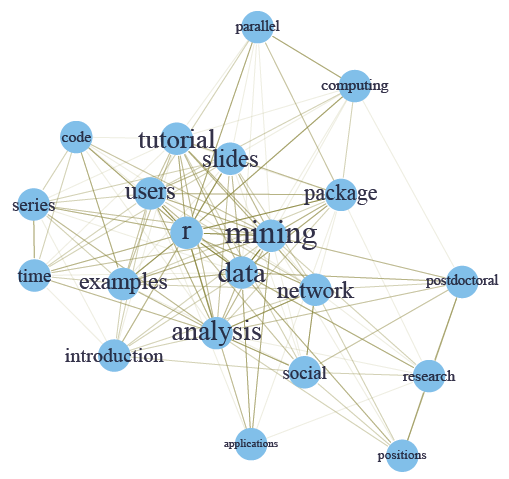
Next, we will set the label size of vertices based on their degrees, to make important terms stand out. Similarly, we also set the width and transparency of edges based on their weights. This is useful in applications where graphs are crowded with many vertices and edges. In the code below, the vertices and edges are accessed with V() and E(). Function rgb(red, green, blue, alpha) defines a color, with an alpha transparency. We plot the graph in the same layout as the above figure.

> V(g)$label.cex <- 2.2 * V(g)$degree / max(V(g)$degree)+ .2 > V(g)$label.color <- rgb(0, 0, .2, .8) > V(g)$frame.color <- NA > egam <- (log(E(g)$weight)+.4) / max(log(E(g)$weight)+.4) > E(g)$color <- rgb(.5, .5, 0, egam) > E(g)$width <- egam > # plot the graph in layout1 > plot(g, layout=layout1)

This presents an example of social network analysis with R using package igraph.  The data to analyze is Twitter text data (sample data). Putting it in a general scenario of social networks, the terms can be taken as people and the tweets as groups on LinkedIn, and the term-document matrix can then be taken as the group membership of people. We will build a network of terms based on their co-occurrence in the same tweets, which is similar with a network of people based on their group memberships.

At first, a term-document matrix is loaded into R. After that, it is transformed into a term-term adjacency matrix, based on which a graph is built. Then we plot the graph to show the relationship between frequent terms, and also make the graph more readable by setting colors, font sizes and transparency of vertices and edges.

Arrange a Conversation